Advanced: Ny-Ålesund Radiation#
In this notebook, we’ll simulate radiation at Ny-Ålesund (Svalbard, 78.9°N) using real radiosonde profiles retrieved from the IGRA database. This demonstrates the complete workflow: fetching atmospheric profiles, converting them to libRadtran format, and running thermal and solar simulations.
import pyradtran
from pyradtran import load_config
import matplotlib.pyplot as plt
import numpy as np
import xarray as xr
from pathlib import Path
import pandas as pd
import logging

# Suppress verbose output from pyradtran
logging.getLogger('pyradtran').setLevel(logging.CRITICAL)

# ── Solar config ─────────────────────────────────────────────────────────────
cfg_solar = load_config()
cfg_solar.simulation_defaults.rte_solver           = "disort"
cfg_solar.simulation_defaults.mol_abs_param        = "reptran per_nm"
cfg_solar.simulation_defaults.source               = "solar"
cfg_solar.simulation_defaults.wavelength_nm        = [400, 3200]
cfg_solar.simulation_defaults.integrate_wavelength = True
cfg_solar.simulation_defaults.output_columns       = ["zout", "lambda", "sza", "edir", "eglo", "edn", "eup", "enet", "albedo"]
cfg_solar.execution.max_workers                    = 16
cfg_solar.execution.cleanup_temp_files             = False
solar_config_path = Path("config/cloud_solar.yaml")
cfg_solar.to_yaml(solar_config_path)

# ── Thermal config ────────────────────────────────────────────────────────────
cfg_thermal = load_config()
cfg_thermal.simulation_defaults.rte_solver           = "disort"
cfg_thermal.simulation_defaults.mol_abs_param        = "reptran medium"
cfg_thermal.simulation_defaults.source               = "thermal"
cfg_thermal.simulation_defaults.wavelength_nm        = [4500, 42000]
cfg_thermal.simulation_defaults.integrate_wavelength = True
cfg_thermal.simulation_defaults.output_columns       = ["zout", "lambda", "sza", "edir", "eglo", "edn", "eup", "enet", "albedo"]
cfg_thermal.execution.max_workers                    = 16
cfg_thermal.execution.cleanup_temp_files             = False
thermal_config_path = Path("config/cloud_thermal.yaml")
cfg_thermal.to_yaml(thermal_config_path)

print(f"Solar config:   {solar_config_path}")
print(f"Thermal config: {thermal_config_path}")

# ── Input dataset ─────────────────────────────────────────────────────────────
N_timesteps = 10
lat, lon = 78.925, 11.922222   # Ny-Ålesund, Svalbard

ds = xr.Dataset(
    coords={
        'time':      pd.date_range('2024-06-07T00:00:00', periods=N_timesteps, freq='1h'),
        'latitude':  ('time', [lat] * N_timesteps),
        'longitude': ('time', [lon] * N_timesteps),
        'altitude':  ('altitude', [0.0]),
    },
    data_vars={
        'surface_temperature': ('time', [275.15] * N_timesteps),  # Kelvin
    }
)

ds
2026-04-19 02:35:06,622 - pyradtran.config - INFO - Configuration written to config/cloud_solar.yaml
2026-04-19 02:35:06,626 - pyradtran.config - INFO - Configuration written to config/cloud_thermal.yaml
Solar config:   config/cloud_solar.yaml
Thermal config: config/cloud_thermal.yaml
<xarray.Dataset> Size: 328B
Dimensions:              (time: 10, altitude: 1)
Coordinates:
  * time                 (time) datetime64[ns] 80B 2024-06-07 ... 2024-06-07T...
    latitude             (time) float64 80B 78.92 78.92 78.92 ... 78.92 78.92
    longitude            (time) float64 80B 11.92 11.92 11.92 ... 11.92 11.92
  * altitude             (altitude) float64 8B 0.0
Data variables:
surface_temperature (time) float64 80B 275.1 275.1 275.1 ... 275.1 275.1Retrieving Radiosonde Data#
We use the RadiosondeAtmosphereGenerator to fetch the closest IGRA radiosonde sounding to our target location and time, then convert it into a libRadtran-compatible atmosphere file.
from datetime import datetime
from pyradtran.io import RadiosondeAtmosphereGenerator

# Build a libRadtran atmosphere file from the closest IGRA sounding
atm_path = RadiosondeAtmosphereGenerator.create_radiosonde_atmosphere_file(
    time=datetime(2024, 6, 7, 0),
    latitude=lat,
    longitude=lon,
    output_filepath="work/sonde_nya.dat",
)

print(f"Atmosphere file created at: {atm_path}")

# Print the first few lines of the generated atmosphere file to verify
print("\nFirst 10 lines of the generated atmosphere file:")
with open(atm_path, 'r') as f:
    for _ in range(10):
        print(f.readline().strip())
Atmosphere file created at: work/sonde_nya.dat

First 10 lines of the generated atmosphere file:
# Radiosonde atmosphere profile
# BJORNOYA at 2024-06-07 00:00 UTC with distance 521.61 km
# p(hPa)  T(K)  h2o(RH%)
11.64  234.45  0.465
12.23  232.85  0.458
13.33  233.45  0.460
13.61  233.55  0.463
14.17  232.15  0.462
14.43  231.75  0.458
14.79  231.65  0.456
Running Simulations#
Now we run both solar and thermal simulations using the radiosonde atmosphere profile. The params argument lets us inject the radiosonde path directly into the configuration.
ds_sim_solar = ds.pyradtran.run(
    config_path=solar_config_path,
    return_dataset=True,
    save_to_file=False,
    params={"radiosonde": str(atm_path) + " H2O RH"},
    show_progress=False,
)

ds_sim_thermal = ds.pyradtran.run(
    config_path=thermal_config_path,
    return_dataset=True,
    save_to_file=False,
    params={"radiosonde": str(atm_path) + " H2O RH"},
    show_progress=False,
)
Results#
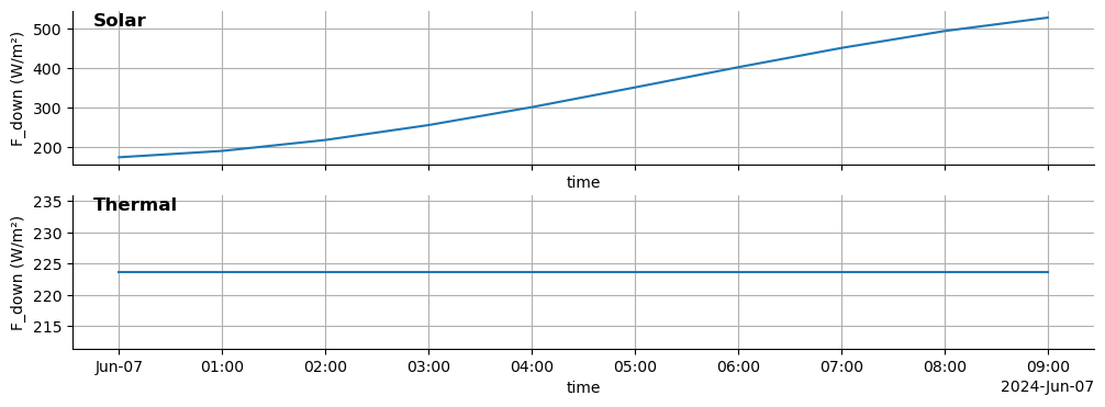
Let’s inspect the simulation output and plot the downwelling irradiance for both solar and thermal spectral ranges.
fig, ax = plt.subplots(2, 1, figsize=(12, 4), sharex=True)

(ds_sim_solar.eglo / 1000).plot(ax=ax[0])
(ds_sim_thermal.eglo).plot(ax=ax[1])

texts = ['Solar', 'Thermal']
for a, t in zip(ax, texts):
    a.text(0.02, 0.9, t, transform=a.transAxes, fontsize=12, fontweight='bold')
for a in ax:
    a.set_ylabel('F_down (W/m²)')
    a.grid()
    a.spines[['top', 'right']].set_visible(False)
    a.set_title('')