Advanced: Reproducing Shupe & Intrieri (2004)#
In this notebook, we’ll attempt to reproduce a key figure from Shupe & Intrieri (2004) — a seminal paper on the Arctic cloud radiative effect. This involves running hundreds of simulations across a grid of cloud parameters to map the relationship between cloud properties and radiative forcing.
Overview#
We assume a standard Arctic winter atmosphere from the libRadtran data directory (
/opt/libRadtran-2.0.6/data/atmmod).This notebook executes hundreds of libRadtran simulations, so it may take a while to run. You can speed it up by reducing the number of parameter steps.
The plot visualizes whether a cloud will cool or warm the surface, and how this depends primarily on the liquid water path (LWP), solar zenith angle, and surface albedo.
import pyradtran
from pyradtran import Var
import matplotlib.pyplot as plt
import numpy as np
import xarray as xr
from pathlib import Path
import pandas as pd
import logging

logging.getLogger('pyradtran').setLevel(logging.CRITICAL)

solar_config_path = Path('config/arctic_cloud_experiment_solar.yaml')
thermal_config_path = Path('config/arctic_cloud_experiment_thermal.yaml')
Cloud Radiative Effect Calculation#
This is an advanced example showing how to perform sensitivity studies on cloud parameters, calculating the cloud radiative effect (CRE) in a libRadtran setup. We calculate the net irradiance for the solar (300–3000 nm) and thermal (3000–100000 nm) bands, under both cloud-free and cloudy conditions.
Surface type |
Shortwave albedo α (broadband) |
Longwave emissivity ε (8–13 µm) |
Notes / typical use |
|---|---|---|---|
Open water |
0.05 – 0.10 |
0.985 – 0.990 |
Low SW reflectance; near-blackbody in TIR |
Thin ice (nilas / young ice) |
0.15 – 0.40 |
0.970 – 0.985 |
Strong thickness dependence; key for leads |
Snow-covered sea ice |
0.75 – 0.90 |
0.980 – 0.995 |
Very high SW albedo; excellent LW emitter |
albedos_sw = np.arange(0, 1.25, 0.25)
albedos_lw = np.arange(0, 1.25, 0.25) * 0  # set to zero (reasonable approximation for high-emissivity surfaces)

# libRadtran handles emissivity as 1 - albedo
albedos_sw
array([0. , 0.25, 0.5 , 0.75, 1. ])
# Arctic stratus parameter space (libRadtran units)
cbh   = [0.3]        # km
cth   = [1.0]        # km

lwps = np.array([5, 20, 50, 100, 400])
lwcs = lwps / 700  # convert to kg m^-3 to fill the 700 m layer uniformly
reffs = [15]

surface_temperatures = np.linspace(273.15, 273.15 - 30, len(albedos_sw))
cbh = [0.3] * len(lwcs)
cth = [1] * len(lwcs)

times = pd.date_range("2024-03-01 12:00", periods=20, freq="7d")
lats = np.arange(80, 60, -1) # this is a trick to sample through a high number of SZA... vary lat and time together...
print(lats)
lon = [0] * len(times)
altitudes = [0, 1, 10, 100]

ds = xr.Dataset(
    coords={
        "time": times,
        "latitude": (("time",), lats),
        "longitude": (("time",), lon),
        "altitude": (("altitude",), altitudes)
    },
    data_vars={
        "lwc": (("lwc",), lwcs),
        "reff": (("reff",), reffs),
        "cth": (("lwc",), cth),
        "cbh": (("lwc",), cbh),
        "surface_temperature": (("albedo",), surface_temperatures),
        "albedo_sw": (("albedo",), albedos_sw),
        "albedo_lw": (("albedo",), albedos_lw),
    }
)

ds_sim_no_cloud_solar = ds.pyradtran.run(
    config_path='config/arctic_cloud_experiment_solar.yaml',
    params={'sur_temperature': Var('surface_temperature'), 'albedo': Var('albedo_sw')},
    save_to_file=True,
    return_dataset=True,
    show_progress=False,
)

ds_sim_no_cloud_thermal = ds.pyradtran.run(
    config_path='config/arctic_cloud_experiment_thermal.yaml',
    params={'sur_temperature': Var('surface_temperature'), 'albedo': Var('albedo_lw')},
    save_to_file=True,
    return_dataset=True,
    show_progress=False,
)

ds_sim_cloudy_solar = ds.pyradtran.run(
    config_path='config/arctic_cloud_experiment_solar.yaml',
    cloud_wc_var='lwc',
    cloud_reff_var='reff',
    cloud_top_var='cth',
    cloud_bottom_var='cbh',
    params={'sur_temperature': Var('surface_temperature'), 'albedo': Var('albedo_sw')},
    save_to_file=True,
    return_dataset=True,
    show_progress=False,
)

ds_sim_cloudy_thermal = ds.pyradtran.run(
    config_path='config/arctic_cloud_experiment_thermal.yaml',
    cloud_wc_var='lwc',
    cloud_reff_var='reff',
    cloud_top_var='cth',
    cloud_bottom_var='cbh',
    params={'sur_temperature': Var('surface_temperature'), 'albedo': Var('albedo_lw')},
    save_to_file=True,
    return_dataset=True,
    show_progress=False,
)
[80 79 78 77 76 75 74 73 72 71 70 69 68 67 66 65 64 63 62 61]
Post-Processing: Cloud Radiative Effect#
Compute the cloud radiative effect (CRE) as the difference between cloudy and cloud-free net irradiance, for both the solar and thermal spectral bands.
ds_sim_no_cloud_solar_normed = ds_sim_no_cloud_solar / 1000
ds_sim_cloudy_solar_normed = ds_sim_cloudy_solar / 1000
ds_cre_solar = ds_sim_cloudy_solar_normed - ds_sim_no_cloud_solar_normed
ds_cre_thermal = ds_sim_cloudy_thermal - ds_sim_no_cloud_thermal
ds_cre_total = ds_cre_solar + ds_cre_thermal
ds_cre_total = ds_cre_total.squeeze()

ds_cre_total = ds_cre_total.assign_coords(
    {'albedo' : albedos_sw}
)
ds_cre_total['enet_zero'] = (('lwc', 'albedo', 'time'), np.isclose(ds_cre_total.enet.isel(altitude=0), 0, atol=.5))
import pandas as pd
import pvlib

def calculate_solar_zenith_angle(time, latitude, longitude):
    solpos = pvlib.solarposition.get_solarposition(times, latitude, longitude)
    return solpos['zenith']
sza = calculate_solar_zenith_angle(ds.time.values, ds.latitude.values, ds.longitude.values)
sza
2024-03-01 12:00:00    87.308757
2024-03-08 12:00:00    83.600046
2024-03-15 12:00:00    79.841690
2024-03-22 12:00:00    76.072131
2024-03-29 12:00:00    72.326330
2024-04-05 12:00:00    68.636291
2024-04-12 12:00:00    65.035708
2024-04-19 12:00:00    61.559141
2024-04-26 12:00:00    58.238263
2024-05-03 12:00:00    55.101745
2024-05-10 12:00:00    52.179414
2024-05-17 12:00:00    49.501237
2024-05-24 12:00:00    47.093743
2024-05-31 12:00:00    44.978874
2024-06-07 12:00:00    43.176652
2024-06-14 12:00:00    41.702779
2024-06-21 12:00:00    40.565954
2024-06-28 12:00:00    39.767156
2024-07-05 12:00:00    39.302199
2024-07-12 12:00:00    39.159366
Freq: 7D, Name: zenith, dtype: float64
ds_cre_total['sza'] = ('time', sza)
ds_cre_sza = ds_cre_total.groupby_bins('sza', [30, 40, 50, 60, 70, 80, 90, 100]).mean()
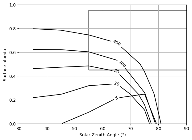
Visualization: CRE Zero-Crossing Contours#
The contour plot below shows the zero-crossing of the net cloud radiative effect as a function of solar zenith angle and surface albedo, for each liquid water path. Lines where CRE = 0 separate the warming and cooling regimes. The rectangle indicates the approximate SHEBA observational domain from Shupe & Intrieri (2004).
fig, ax = plt.subplots(figsize=(7, 5))

colors = plt.cm.inferno(np.linspace(0, 1, len(ds_cre_total.lwc)))

for i, lwc in enumerate(ds_cre_total.lwc.values):

    cs = ds_cre_sza.isel(altitude=0).sel(lwc=lwc).enet.plot.contour(x='sza_bins', colors='k', levels=[0])
    # add lwc to complete the label
    cs.clabel(fmt=f'{lwps[i]}', colors='k')

# show SHEBA region
from matplotlib.patches import Rectangle

ax.add_patch(Rectangle((55, .45), 50, .5, alpha=0.5, edgecolor='k', linewidth=2, fill=False))

ax.set_xlim(30, 90)
ax.set_ylim(0, 1)
ax.set_title('')
ax.grid()
ax.set_xlabel('Solar Zenith Angle (°)')
ax.set_ylabel('Surface albedo ')
Text(0, 0.5, 'Surface albedo ')
Extension: Ice Cloud Simulations#
Below, we repeat the analysis using ice water content (IWC) instead of liquid water content, to explore the radiative effect of ice clouds.